Synthesizing information with PivotTables in Excel (Pivot)
have a rather large table and different perspectives need to extract the information it contains. For example, a table of cars, drivers, miles and consumption sometimes need to know how many miles does a driver in particular and other how much consumption a specific car. Or have a table of review documents to be drawn which are of an author or a topic ... Or give you a huge table and ask you what customers have such a product? and after a while they ask you what products have such a client? (Sunday, March 27, 2011
How To Increase Money In Pokemon Deluge
from a table where each column has its unique title. We are in a column if the subject is Darn Right or (d / z), in another gender (v / m) and a third a unique identifier for each. Do not ye break the head of the table data to me just invented on the fly. Select all data, header included
 and give "Data"> "Tables and Graphs Report dynamic. "
Sale
 a wizard, accept the defaults and give you a complete directory ...
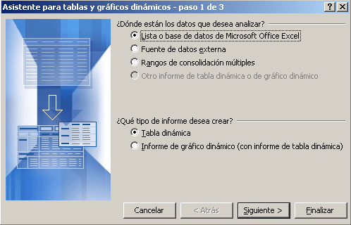
... and the titles of the columns, such as drag indicated in the image (this is already aunue to consumer tastes, this is the creative part of the pivots)

already have the table. There is a problem, and the result is meaningless because their added values \u200b\u200bof the identifiers for each user. We changed the "sum" for the simple "count" identifiers (Other possible functions are Count, Average, Min, Max, Product ...)

already have the table

In seconds we obtained a summary table we can see at a glance key information from the original table, and answer many questions out we can do about the same how many men were involved? How many left-handed subjects? How many skilled women? Double click on any of the values \u200b\u200band create a new table with only those records that meet that condition. Click on the icon of graphs and takes us a graphic interpretation of the data. Play with it. Another day I speak of Solver and Excel scenarios.

Another good example TodoExpertos . Remember, Google is your friend . The historical data . As always, thanks for coming . If you liked the post you can subscribe via e-mail or via RSS feed ( more about RSS ). You can also follow through my Google Reader shared items and from Twitter.
Subscribe to:
Post Comments (Atom)
0 comments:
Post a Comment